What is GAN?-Counterfeiter and Policeman 🚓

The GAN (Generative Adversarial Nets) model is a model that lets you learn how to create results by competing two opposing neural networks. The dictionary meaning of the word “adversarial” has the meaning of confrontation and opposition. In order to confront, you have to have an opponent anyway, so you can intuitively know that GAN is largely divided into two parts.

By Tim O’Shea, O’Shea Research.

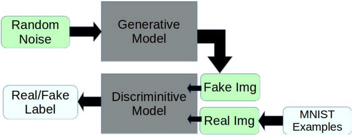
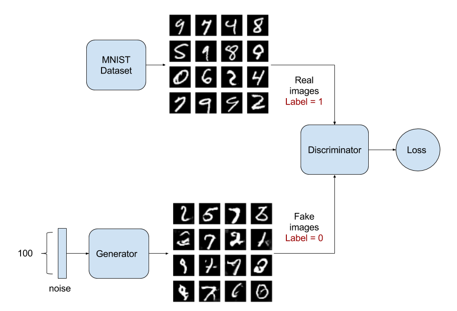
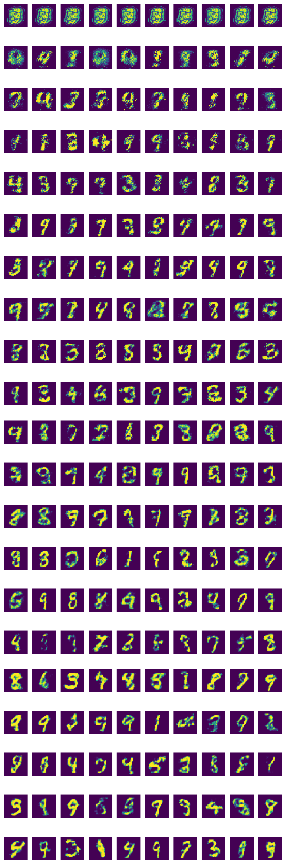
Some of the generative work done in the past year or two using generative adversarial networks (GANs) has been pretty exciting and demonstrated some very impressive results. The general idea is that you train two models, one (G) to generate some sort of output example given random noise as input, and one (A) to discern generated model examples from real examples. Then, by training A to be an effective discriminator, we can stack G and A to form our GAN, freeze the weights in the adversarial part of the network, and train the generative network weights to push random noisy inputs towards the “real” example class output of the adversarial half.

Fig.00 - Conceptual diagram of GAN model
[REF:]: MNIST Generative Adversarial Model in Keras

1.0 Counterfeiters are becoming more intelligent by competing.

According to the analogy presented by Ian Goodfellow, who proposed the GAN model, the counterfeiter (producer neural network) and the policeman (constituent neural network) oppose each other, and the police try to discriminate, and the counterfeiter is counterfeit. It is to learn how to make high-quality counterfeit bills that are difficult to distinguish from the real through the relationship that advances the method.

Fig.00 - Conceptual diagram of GAN model
[REF:]: MNIST Generative Adversarial Model in Keras

2.0 to Create GAN model using MNIST

• At first, it generates a simple noise like character, can’t understand.
• As it goes through the learning, you can begin to identify the counterfeit imitation
• And As much going further it is gradually becoming concrete.

Fig.01 - At first, the generator is anything, just throwing it away… it’s just a noise!

Fig.02 - As the iterations repeat, the imitation becomes more detailed.

Fig.03 - It has become quite sophisticated. Now it’s only 300 iterations

Fig.04 - The elaboration process has ended when it has already exceeded 1,000 times.

3.0 Comparison of the original and counterfeit results

• In fact, the handwriting shown here is a completely brand new imitated handwriting data that MNIST doesn’t have.
• Only a Created Data Which is not exist in the real world!!

01.the original	02.the counterfeit

2.0 The whole process that the real-like imitations are being made.

• shopisticate correction was being achieved over 100 times of learning iterations for each image.
• After almost about 1,000 times, the elaboration process seems to be over. (which one is copy?)

Fig.04 - imitation of handwriting is being shopisticate with feedback through competitions

3.0 References

1. MNIST Generative Adversarial Model in Keras
2. Jaejun Yoo’s Playground: Easy to Understanding the Generative Adversarial Nets
3. hacker’s 3-minutes lecture : Deep learning - tensorflow taste …. ( hanvit-media / Kim Jin-Jung )

CODE PART.01 - definition of Variables

import os
import sys
import tensorflow as tf
import matplotlib.pyplot as plt
import numpy as np

# Set 'root-dir' and 'working-dir' - for Atom Environment, Script-Run
DIRS = os.path.dirname(__file__).partition("deep_MLDL")
ROOT = DIRS[0] + DIRS[1]
sys.path.append(ROOT)

from os.path import dirname, join
WORK_DIR = join(ROOT,'_ static','MNIST_data','')


from tensorflow.examples.tutorials.mnist import input_data
mnist = input_data.read_data_sets(WORK_DIR, one_hot=True)

 # Hyper- Parameter
learning_rate = 2e-4
training_epoches = 100
batch_size = 100

n_hidden = 256
n_input = 28*28             # 784 pix. for 1 letter
n_noise = 128

 # placeholder
X = tf.placeholder(tf.float32, [None, n_input])
Z = tf.placeholder(tf.float32, [None, n_noise])

G_W1 = tf.Variable(tf.random_normal([n_noise, n_hidden], stddev=0.01))
G_b1 = tf.Variable(tf.zeros([n_hidden]))

G_W2 = tf.Variable(tf.random_normal([n_hidden, n_input], stddev=0.01))
G_b2 = tf.Variable(tf.zeros([n_input]))

D_W1 = tf.Variable(tf.random_normal([n_input, n_hidden], stddev=0.01))
D_b1 = tf.Variable(tf.zeros([n_hidden]))

D_W2 = tf.Variable(tf.random_normal([n_hidden, 1], stddev=0.01))
D_b2 = tf.Variable(tf.zeros([1]))

CODE PART.0 - function definition

def generator(noise_z):
    hidden = tf.nn.relu(tf.matmul(noise_z, G_W1) + G_b1)
    output = tf.nn.sigmoid(tf.matmul(hidden, G_W2) + G_b2)
    return output

def discriminator(inputs):
    hidden = tf.nn.relu(tf.matmul(inputs, D_W1) + D_b1)
    output = tf.nn.sigmoid(tf.matmul(hidden, D_W2) + D_b2)
    return output

def get_noise(batch_size, n_noise):
    return np.random.normal(size=(batch_size, n_noise))

CODE PART.03 - the variable definition

G = generator(Z)
D_gene = discriminator(G)
D_real = discriminator(X)

cost_D = tf.reduce_mean(tf.log(D_real) + tf.log(1-D_gene))
cost_G = tf.reduce_mean(tf.log(D_gene))

D_var_list = [D_W1, D_b1, D_W2, D_b2]
G_var_list = [G_W1, G_b1, G_W2, G_b2]

train_D = tf.train.AdamOptimizer(learning_rate).minimize(-cost_D, var_list=D_var_list)
train_G = tf.train.AdamOptimizer(learning_rate).minimize(-cost_G, var_list=G_var_list)

CODE PART.04 - draw a graph

# Draw Graph - Neural Networ training
init = tf.global_variables_initializer()
sess = tf.Session()
sess.run(init)

total_batch = int(mnist.train.num_examples / batch_size)
loss_val_D, loss_val_G = 0, 0

for epoch in range(training_epoches):
    for i in range(total_batch):
        batch_xs, batch_ys = mnist.train.next_batch(batch_size)
        noise = get_noise(batch_size=batch_size, n_noise=n_noise)

    # calculate train(optimize), cost function as pair
    _, loss_val_D = sess.run([train_D, cost_D], feed_dict={X:batch_xs, Z:noise})
    _, loss_val_G = sess.run([train_G, cost_G], feed_dict={Z:noise})

    if epoch%10 == 0:
        print("Epoch:%3s ___ Cost_D: %.9f"% (epoch, loss_val_D))
        print("          ___ Cost_G: %.9f\n"% (loss_val_G))

    # Check generated image
    if epoch == 0 or (epoch+1)%10 == 0:
        sample_size = 10
        noise = get_noise(sample_size, n_noise)
        samples = sess.run(G, feed_dict={Z:noise})
        fig, ax = plt.subplots(1, sample_size, figsize=(sample_size, 1))

        for i in range(sample_size):
            ax[i].set_axis_off()
            ax[i].imshow(np.reshape(samples[i], (28, 28)))

        plt.savefig(WORK_DIR + '{}.png'.format(
            str(epoch+1).zfill(3)),
            bbox_inches = 'tight')
        plt.close(fig)

print('...optimizing finished ...')

Written on ... September 17, 2018